Graphing Calculator
for Macintosh and Windows
What's new in Version 5.0 for macOS & iOS
- Version 5 has made substantial improvements in Graphing Calculator's ability to simplify and solve equations
- Symbolically evaluate integrals, summations, products, and limits
- Simplify and expand trig identities
- Solve equations, systems of equations, inequalities, and differential equations symbolically
- Factor polynomials
What's new in Version 4.1 for macOS
- 64-bit binary
- Sliders for point radius and line width
- Select vector and matrix elements by subscript
- Allows slider variables in set definitions
- Support arrows and complex points on right hand graph pane in split views
- Support trackpad for zoom on 2D graph views
- Removed 4D graphing
What's new in Version 4
- Tables
- Graphing data
- Graphing 3D points
- Graphing surfaces of revolution
- Graphing ordinary differential equations in 3D
- Specify ODE initial conditions
- Tube plots
- Numeric Integration
- New functions
- Long variable names
- Universal binary on Mac OS X
- Support for multiple processors
What was new in Version 3.5
- Subscripts
- Parameter sets
- Native Mac OS X application
What was new in Version 3.2
- Vectors
- Coordinate Transformations
- Free Viewer application available on Mac and Windows
What was new in Version 3.1
- Complex numbers
- Complex number arithmetic
- Complex function parametric curves in 2D
- Complex function parametric curves in 3D
- Complex function surfaces in 3D
- Complex function surfaces in 3D with color coding
- Complex function surfaces in 4D
- Interactive complex parameters
- Color maps in 2D
- Point plots in 2D
- Vertex lists in 4D
- Parametric curves in 4D
- Parametric surfaces in 4D
- Examples menu and sample documents
- New functions
- Text expressions in coordinate ranges
- Direction fields
What was new in Version 3.0
- Text comments in documents
- Printing
- Multiple document windows
- Save as web page
- Save as RTF for export to word processors
- 3.0 acts as a helper application for GC documents posted to the web
What was new in Version 2.7
- Change the 3D background color
- Define functions and variables symbolically
- Copy and paste formulas as plain text
- Equations now line-break and scroll
- 1st order ordinary differential equations in 2 dimensions
- Correct handling of fractional powers
- New functions
Tables
You can enter tables of data, numerically transform the data, and graph data in two and three dimensions.
Surfaces of revolution
You can rotate a curve around an arbitrary axis to generate a surface in three dimensions.
3D Ordinary Differential Equations
You can graph ODEs in three dimensions.
You can specify initial conditions for ODEs by giving starting points on surfaces.
Tube plots
Numeric integration
Binomial coefficient
Products
Matrix operations
Complex Conjugate
Logical expressions
Vector fields
Vector fields can be graphed on surfaces.
Parameter sets
2D Vectors
3D Vectors
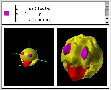
Coordinate Transformations
Complex number arithmetic
You can use Graphing Calculator 3.1 as a calculator for complex numbers. For example:
Complex function parametric curves in 2D
A complex function of a real parameter, t, specifies a curve in 2D. For example:
This is a shorter way of writing the parametric equation:
You can also use z as shorthand for x + iy. For example:
Complex function parametric curves in 3D
A complex function of a real parameter, z, specifies a curve in 3D. Observe that this is the same complex function as in the 2D example above, but here the parameter z is used as the third 3D coordinate.
This is similar to writing the parametric equations:
Parametric curves in 4D
You can also write parametric equations for curves in four dimensions by specifying functions (which have real values) for each of the four spatial coordinates x, y, u, and v. For example:
Complex function surfaces in 3D
Using z as shorthand for x + iy, you can graph 3D surfaces representing complex functions. For example:

In this example, observe the four zeros at +1, -1, +i, and -i.
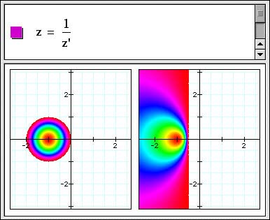
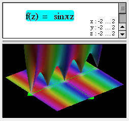
Complex function surfaces in 3D with color coding
Using z as shorthand for x + iy, you can graph 3D surfaces representing complex functions. The height of the surface represents the magnitude of the complex function. The phase of the complex function is encoded in the color of the surface. For example:
Complex function surfaces in 4D
A complex function f(x + iy) depends on two real parameters x & y and has two components, Re f, and Im f. We can render this as a surface in 4 spatial dimensions with coordinates:
(x, y, Re f(x+ iy), Im f(x + iy)) and then project this surface to the screen in a manner similar to the way we project 3-D surfaces onto a 2-D screen. Note that in the following, z=x+iy and w=u+iv.
Interactive complex parameters
In the following example, you can drag the purple dot, which moved the square grid along with it. The blue grid is the map of the square grid under the complex function f(z).
Color maps
You can specify the color at each point in the place by giving functions for either the (red, green, blue) or the (hue, saturation, value) components of the color.
Point plots
In the following example, as n varies, the point traces out a circle:
Vertex lists in 4D
The following shows a hypercube in four dimensions specified by writing the 32 edges between its 16 vertices.
Parametric surfaces in 4D
This is the parametrization for a flat torus in 4D. It is the product of an x-y circle (sin u, cos u), and a u-v circle (sin v, cos v). (The four 4D coordinate axes are x, y, u & v. The letters u & v are also used separately for the surface parametrization. This is confusing as u and v must be interpreted differently depending on context.)
New functions
The min() function returns the minimum of its arguments.
The max function returns the maximum of its arguments.
mod(a,b) return the remainder of a divided by b.
clamp(x,a,b) pins x to the range [a,b].
Text expressions in coordinate ranges
Direction fields
Type command-option-d to draw unit vectors in a vector field.
Examples menu and sample documents
Version 3.1 ships with example and template documents which are also accessible from the new Examples menu.
Background Color
The preferences dialog now gives control over the background used with 3D objects.
Defining variables and functions
(You must type "f control-9 x" to distinguish f(x) as a function.)
Copy and Paste formulas as plain text
Copy as Text on  produces sum(x^k/k!,k=0,5).
Equations line-break and scroll
1st order 2D ordinary differential equations
Fractional powers
Fractional powers of negative numbers are handled properly now.
Bessel functions
Floor and ceiling
Piecewise defined functions
Div, grad, and curl

Vector dot and cross products
Summations
Substitutions
New releases
If you would like to help test pre-release development versions of our products, subscribe to our mailing lists here.
